
A Koala’s Guide to Factor Investing
In my article, Why index funds are the optimal place to start, the academic literature suggests the average person should start with index funds. So what should a person who is not average do?
Ignoring the philosophical question on what it means to be “average,” if someone is uncomfortable with having all their investments in index funds, then it makes intuitive sense for them to hold more defensive assets like bonds or cash. But what to do if someone believes they can handle more risk?
They could either do some form of leveraging or apply factor investing to their portfolio. To answer what factor investing is, it’s best if I go through the academic history that led to the emergence of factor investing.
Before I go on, this is supposed to be an “introduction” to factor investing, but for those who are more experienced, I’ve included a couple bits of additional information that are not necessary to know but are interesting nonetheless. Below is an example:
Where to learn more?
For those who are interested in learning more or have questions about factor investing, the Rational Reminder Community would be the best place to do so. The community is also generally the hub for discussions on academically driven investing: Rational Reminder Community
If you want to read more articles relating to factor investing, AlphaArchitect is a great website to do so. Their business is offering ETFs (which I am not necessarily endorsing), but the wealth of information they provide for free through summarising papers and writing articles is immensely helpful: Alpha Architect.
History
To get the necessary context, I’ll first start with the Capital Asset Pricing Model (CAPM). I’ve previously mentioned CAPM in my article on Why index funds are the optimal place to start, but I’ll explain it in more detail here. Below is a regression that stems from the CAPM formula:
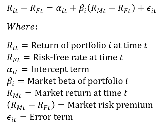
What the regression aims to achieve is to explain the returns and risk of an asset or portfolio to the market. This is done by using market beta to measure the returns and risk of a portfolio relative to the market. For example, if the market beta for a portfolio is 1.2, then the portfolio has more risk than the market and a higher return. If the market risk premium was 10% over a time period, the portfolio with a market beta of 1.2 would return 12%. If over another time period the market risk premium was -10%, then the portfolio would return -12%. If the market beta was less than 1, then the portfolio would be less risky than the market and have a lower return. When the market beta equals 1, this could mean the portfolio is the total stock market portfolio but does not necessarily need to be.
Now, CAPM, a one-factor model, assumes that alpha equals zero in the regression, an assumption that poorly reflects reality, seeing that the model could only explain roughly two-thirds of a portfolio’s return. An example of using CAPM to analyse the cross-section of a portfolio’s return (in other words, the difference in returns between portfolios) is if portfolio A had a return of 10% and portfolio B had a return of 13%, then of the 3% difference in returns, CAPM could only attribute 2% to differences in market beta with the remaining 1% assumed to be luck or skill of the manager. However, over the following decades, researchers have been finding anomalies that could not be explained by market beta. This gave rise to the Fama-French 3 Factor model (FF3) formulated by Fama and French (1992), which added two additional factors: Size and Value. The Size factor is the tendency for small stocks to have higher returns than larger stocks, first documented by Banz (1981) and Reinganum (1981). On the other hand, the Value factor is the tendency for cheap stocks to have higher returns than expensive stocks, first documented by Basu (1977).
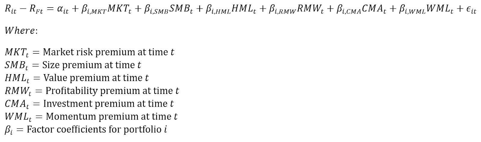
The FF3 is now able to explain more than 90% of a portfolio’s return. But it didn’t stop there. Carhart (1997) added Momentum to the model, first documented by Jegadeesh and Titman (1993), now explaining about 95% of a portfolio’s return. In 2015, Fama and French then formulated the Fama-French 5 Factor model (FF5) by adding two additional factors: Profitability (Novy-Marx, 2013) and Investment (Titman et al., 2004). Fama and French (2018) then reluctantly added Momentum to create the Fama-French 6 Factor model (FF6). This gives the regression shown below:
Q-model
Fama and French aren’t the only ones to create asset pricing models. The most popular alternative is the Q-model, first conceived by Zhang and Chen (2007) as a three-factor model consisting of market beta, profitability, and investment. Hou, Xue, and Zhang (2015) then added size as a factor, resulting in a four-factor model. What differentiates the Q-model is first laying an economic and theoretical foundation for what drives a stock’s return and then testing their model with data. This is opposed to Fama and French doing the opposite approach of first trying to explain a stock’s return using data and then thinking of the theoretical reasons why. This not only led to the Q-model having a more robust theoretical argument but also explained returns better than FF3 and FF4. Although the Q-model is pretty similar to the FF5, it is able to perform better than the FF6 when Hou, Mou, Xue, and Zhang (2021) added the expected growth factor.
The weaknesses of the Q-model include dismissing behavioural-based explanations of risk and being less practical to implement in the real world because of the higher turnover. This is evidenced by Detzel, Novy-Marx, and Velikov (2021), finding that the FF5 performs better than the Q4-model when taking transaction costs into account.
With the FF6 model in mind, below is how I like to define factor investing.
Factor investing: the targeting of independent, risk-premia factors as a way to achieve returns above the market return and/or increase portfolio diversification.
What do I mean by independent, risk-premia factors? The easiest way to explain this is to learn how to interpret factor regressions.
How to read factor regressions
Below is a simplified version of the FF3 regression over some time period:

The beta coefficients in the regression are called factor loadings, and as a reminder, MKT is the Market factor premium, SMB is the Size factor premium, HML is the Value factor premium, and alpha is any unexplained return.
Let’s take a total stock market (TSM) portfolio as an example (the equivalent ETFs would be VAS or A200 for the Australian market and DHHF for the global market). By definition, the TSM portfolio will have a Market factor loading of exactly 1 with all other factor loadings equaling 0. This means that the return of a TSM portfolio equals the return of the Market factor plus alpha (alpha in this case will be negative because of ETF fees). Now, the premiums for the Size and Value factors may be positive over this period, but we don’t get any exposure because the factor loadings equal 0.
Let’s take another portfolio, but this time let’s have the factor loadings for Size and Value equal 0.5 and keep the Market factor loading as 1. As an example, let MKT = 5%, SMB = 2%, HML = 3%, and alpha = 0. Then:

Going back to the definition of factor investing, risk-premia factors are making the factor loadings positive (excluding the Market factor) so that the portfolio’s return gets positive exposure to factors other than the Market factor. This simple example also demonstrates how factor investing can achieve returns above the market through the exposure of beta factors rather than trying to rely on alpha (luck or skill).
Let’s take another example, keeping the loadings the same but with different premiums:

This example demonstrates factors being independent from each other, where the factor premiums may not move up or down in the same way. This is also why factor investing can offer a diversification benefit to a portfolio. As in the example above, a TSM portfolio would’ve had a -5% return over the time period, whereas the factor-tilted portfolio had a 0%. Just note that it isn’t always sunshine and rainbows with factor investing. There can be times when factors can go through long periods of underperformance relative to a TSM portfolio. That’s what makes factors risky.
Now that we solidified our understanding of what risk-premia factors are and why they are independent, it is now a good time to go through what factors are exactly.
Factor loadings vs. characteristics
After creating the FF3 model, Fama and French (1993) argued that factor loadings indicate how much exposure you have to certain risks, so a higher loading means more risk and return. This goes against possible behavioural-based explanations for factors, such as Lakonishok et al. (1994) for the value factor. It also raises the question of whether factor loadings are the best way to explain cross-sectional return variation. Rather than using factor loadings, Daniel and Titman (1997) argued that characteristics do a better job of explaining cross-sectional return variation than factor loadings. In other words, the characteristics of a portfolio (book-to-market ratio or market cap) are more predictive of expected returns than the portfolio’s factor loadings on HML or SML. There has been debate over factor loadings vs. characteristics since Daniel and Titman’s paper, but there appears to be stronger evidence for the characteristics camp (Gray, 2024).
This is all to say that there is nothing wrong with using factor regressions to compare two funds. But there are weaknesses that come with factor regressions to keep in mind, and in an ideal world we can use both factor loadings and current characteristics to compare funds, as suggested by Jack Vogel in his article, Do Portfolio Factors or Characteristics Drive Expected Returns?
What are factors?
There are two categories of factors: macroeconomic factors and style factors. Examples of macroeconomic factors are GDP, inflation, and interest rates. We can’t control macroeconomic factors, and so we are more interested in style factors, more specifically style factors related to stocks. The most popular style factors are in the FF6 model: Market risk, Size, Value, Profitability, Investment, and Momentum.
Below is how the returns for each factor get measured:
- Market risk – stock returns minus bond returns.
- Size (SMB) – the return of small companies minus the return of big companies.
- Value (HML) – the return of high book-to-market value ratio companies (cheap companies) minus the return of low book-to-market value ratio (expensive companies).
- Profitability (RMW) – the return of companies with robust profitability minus the return of companies with weak profitability.
- Investment (CMA) – the return of companies that invest conservatively minus the return of companies that invest aggressively.
- Momentum (WML) – the return of recent winners minus the return of recent losers.
This was how academics defined factors by measuring the gap between the two extremes. The extreme that has historically resulted in higher returns is referred to as the long leg, while the extreme with lower returns is the short leg. In academic research, factors are typically defined as long/short or long minus short, as it makes analysis easier. But in the context of investing, factor funds are referred to as long only, which is just a fancy way of saying a fund overweights companies with desirable characteristics associated with risk-premia factors.
To be considered a risk-premia factor, the factor must meet all of the following criteria proposed by Larry Swedroe and Andrew Berkin in their book Your Complete Guide to Factor-based Investing:
- Persistent – holds over long time periods and different economic regimes.
- Pervasive – holds across countries, sectors, and other asset classes.
- Robust – holds over multiple definitions.
- Intuitive – there are risk and behaviour explanations for its existence.
- Investable – holds after accounting for real-world fees.
Persistent and Pervasive
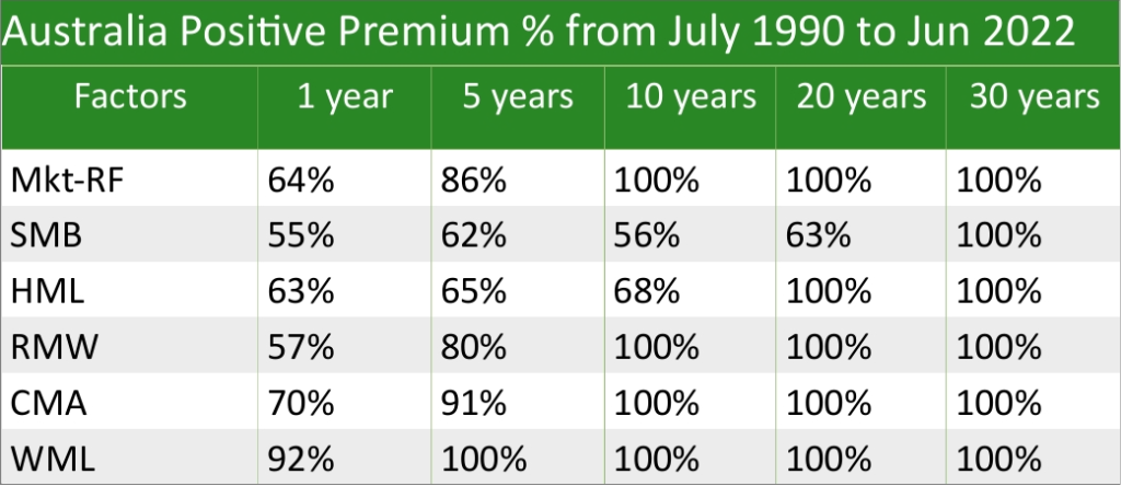
To demonstrate the persistence of the six premia factors, the table below shows the percentage of a positive premium for long/short factors (i.e., the long side beating the short side) over rolling X years from July 1963 to August 2024 for the US. For those who don’t know what rolling years are, examples of rolling 1-year periods are: 07/1963 – 06/1964, 08/1963 – 07/1964, 09/1963 – 10/1964,…, and 09/2023 – 08/2024.
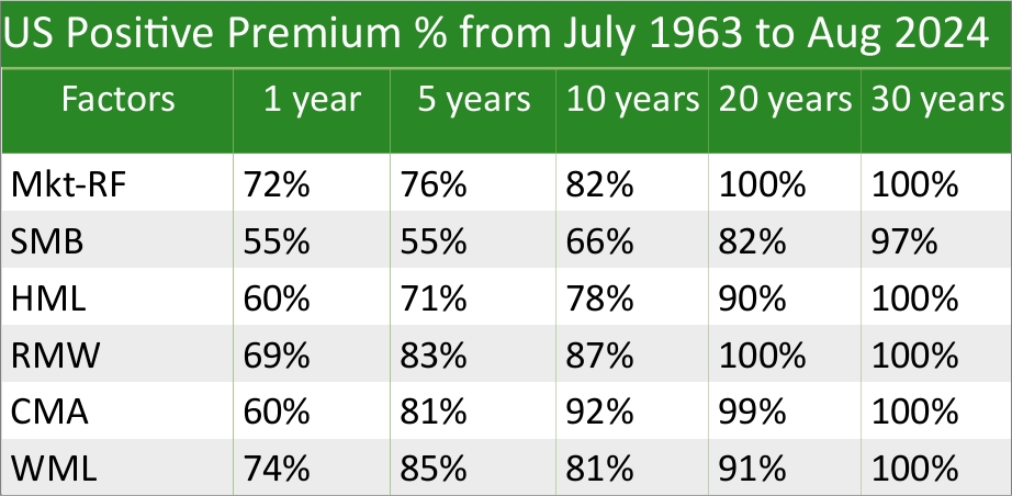
I used Kenneth R. French data [Fama/French 5 Factors (2×3)] which excludes transaction costs. So keep in mind that the analysis of risk-premia factors will look better than how they’d actually do live, especially for high-turnover factors like Momentum (WML).
To demonstrate pervasiveness, using data from Global Factor Premia, which also excludes costs, the tables below show global ex-US and Australia from July 1990 to June 2022 (note that this is a significantly shorter time frame than the US data).
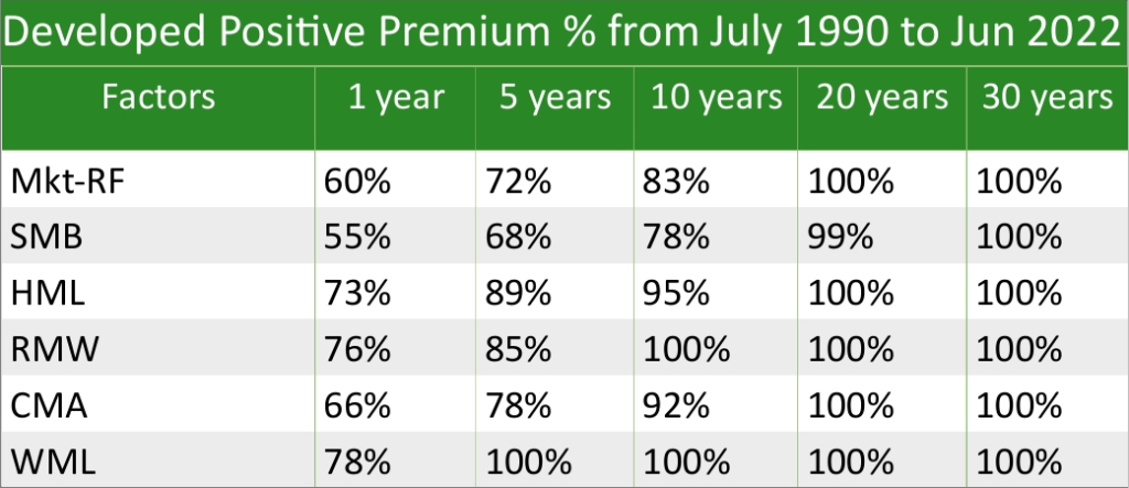
Furthermore, factors are found to exist in other asset classes like bonds, commodities, currencies (Asness, 2013; Ilmanen et al., 2021), and cryptocurrencies (Akbari et al., 2024), as well as other markets such as sports betting (Moskowitz, 2021) and LEGO sets (Shanaev et al., 2020).
Robust and Intuitive
The below table shows examples of different definitions for each factor to demonstrate robustness, as well as showing that these factors are intuitive with risk-based and behavioural-based explanations that have been proposed by academics (I’d like to credit Wiest’s (2022) paper summarising the literature on Momentum over the last 30 years, which helped me get risk and behavioural-based explanations for Momentum).
| Factor | Definitons | Risk-based explanations | Behaviour-based explanations |
|---|---|---|---|
| Value |
|
|
|
| Size |
|
|
|
| Profitability |
|
|
|
| Investment |
|
|
|
| Momentum |
|
|
|
HOWEVER, the decades of cumulative research I presented above (as well as my time spent putting it all together) might be all in vain with the recent paper, Does Peer-Reviewed Research Help Predict Stock Returns? by Chen et al. (2024). In the paper, they data-mined (the process of trying every single combination) 29,000 accounting ratios, took those that are statistically significant, and compared them to peer-reviewed factors. What they found was that their data-mined factors had similar post-sample returns to peer-reviewed factors. On top of this, peer-reviewed factors with risk-based explanations underperform, and factors with the most rigorous theory had the worst post-sample performance. The conclusions sound grim, but the authors try to end the paper on a hopeful note:
“We do not argue economists should become engineers and abandon elegant and parsimonious theories. Such theories are our strength—they are the very meaning of the expression “the economics.” Instead, we argue that data mining could be the key to ensuring our theories stay relevant. Put another way, completely exploring the data should lead to theories that are closer to the fundamental sources of returns of the real world.”
Investable
Okay, maybe factors aren’t as intuitive as we first thought they were, but can they still be applied to the real world? Given how reliable and easy to understand passive investing is, we can unanimously agree that the market factor is investable. But what about the other factors?
This is still a widely contested topic that tries to get to the bottom of two questions:
- How much have factor premiums decayed since they were first published? Now that factors are more widely known, more investors will be putting their money into these factors, lowering the factor premiums.
- Does the premium survive after transaction costs? Transaction costs can include commissions, bid/ask spreads, turnover costs, and price impact. Price impact is when a fund trades a stock and there is not enough volume on the other side of the trade, causing an impact on the price. This effect worsens the larger the fund is, and eventually there is a point when the fund no longer has enough capacity to still earn a premium.
How much decay?
McLean and Pontiff (2016) found a 32% decay from publication-informed trading and a total 58% post-publication decay in the US market, where they found the decay to be larger for factors that are less costly to arbitrage (more liquid stocks and less volatile stocks). This finding is supported by Calluzzo et al. (2019).
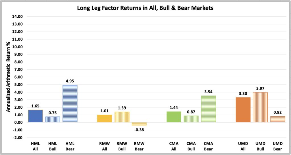
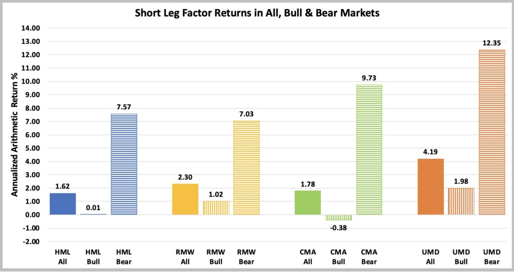
However, Blitz (2023) and Geertsema and Lu (2022) finds that most of the returns of factors are generated during bear markets. This suggests mispricing builds up during bull markets and gets corrected during bear markets. This finding also explains the lower performance of factors, where Blitz found bear markets to occur 27% of the time before 2004 and 9% of the time after 2004. Because of this, the 67% performance decay after 2004 becomes 33% after accounting for less frequent bear markets. Outcast Beta’s article, Dissecting factor returns in bull and bear markets, shows two graphs showing factor returns in bear and bull markets for the long leg and short leg separately in the US market from 1963 to 2021:
Furthermore, Jacobs and Müller (2020) find that the decay was only statistically significant in the US market, while the same cannot be said for the international market. This contradicts Zaremba et al. (2021), who found decay in the international markets as well.
Reasons for this decay have been theorised to be caused by:
- Increase in liquidity:
- For: Chordia et al. (2014) and Brogaard et al. (2024).
- Against: Calluzzo et al. (2019) and Auer & Rottmann (2018).
- Arbitrage trading:
- Data snooping:
- For: Linnainmaa and Roberts (2018) and Hou et al. (2017)
- Against: Jacobs and Müller (2020)
Do factor premiums survive?
Yes
- Frazzini et al. (2014), using over a trillion dollars of live data from AQR spanning 1998 to 2011, found Value, Size, and Momentum survive after transaction costs. They further claim that the maximum capacity of global funds would be $1.8 trillion for Size, $811 billion for Value, and $122 billion for Momentum. The findings of this study that used live data contrasted previous research, as academic models tend to overestimate costs.
- Novy-Marx and Velikov (2014) also come to the conclusion that factors such as Size, Value, Profitability, Momentum, and Investment can survive after costs, especially when utilising cost mitigation strategies.
- Ratcliffe et al. (2017) (researchers from Blackrock) find the capacities for factors from 1975 to 2016, assuming a 50% decay, are $2.5 trillion for Size, $153 billion for Value, $27 billion for Momentum, and $151 billion for a Multifactor fund. However, when spreading the trades across five trading days, capacities increase to $12.4 trillion for Size, $763 billion for Value, $136 billion for Momentum, and $754 billion for a Multifactor fund.
- Ross et al. (2017) used AQR Momentum funds from 2009 to 2016 to find that Momentum is implementable after costs.
No
- Chen and Velikov (2021) argue that using data dating to the 1900s would be irrelevant when future returns will be much smaller with the knowledge and technology we have in today’s age. To create a more realistic scenario, they only used data post-2005 and found expected returns of anomalies to be close to zero after accounting for trading costs. Andrew Chen does note on The Rational Reminder Podcast that although targeting single factors may not yield a premium after costs, combining factors may still yield a return after costs.
Although Chen and Velikov’s findings may seem defeating, keep in mind Blitz’s findings about factor returns and bear markets being less frequent after 2004 and the tendency for academics to overestimate costs. Even if factor returns are zero, factors are still beneficial for providing a diversification benefit.
Diversification
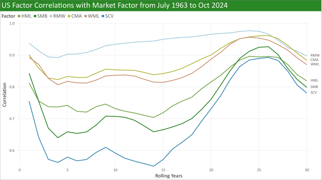
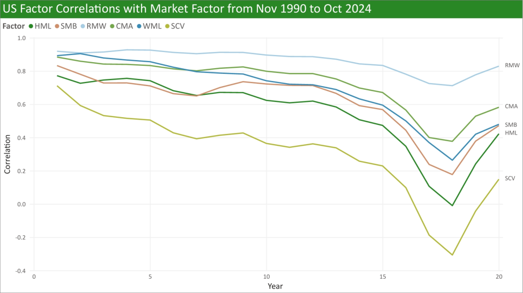
Factors can offer a diversification benefit because of their imperfect correlation with the market over time. Below shows the correlation of long-only factors (also including Small-Cap Value or SCV) with the market over rolling years for the US (all analysis in this section uses Kenneth R. French’s data and so excludes transaction costs):
Below is the same but for developed markets:
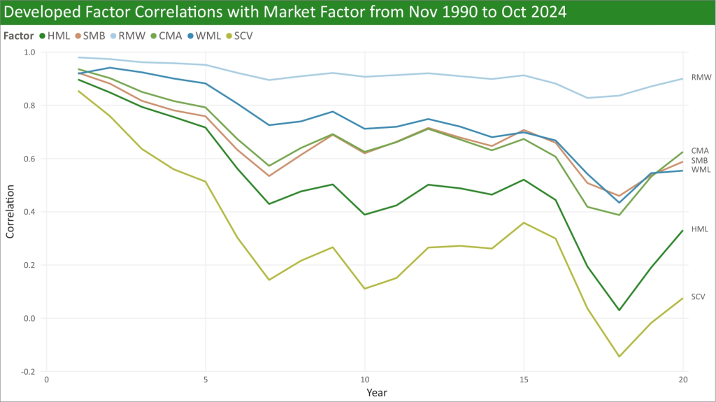
Value and SCV’s correlation going as low as 0 is wild, but this is because of the short time period analysed and the dominance of risk-premia factors within this period. Below is the US again but over the same time period as Developed, showing similar results:
ERN recently wrote an article dismissing the diversification benefits of factors, specifically small cap value, and I would like to talk about one of the points they made. They argue that the diversification benefits of small cap value are “statistically false” because the standard deviation of the market is less than the standard deviation of SCV multiplied by their correlation, implying that adding SCV to a portfolio would only increase the portfolio’s volatility. This does seem true if you calculate correlations and standard deviations from 1-year returns, but not when using longer rolling years, as shown in the table below from July 1963 to Oct 2024:
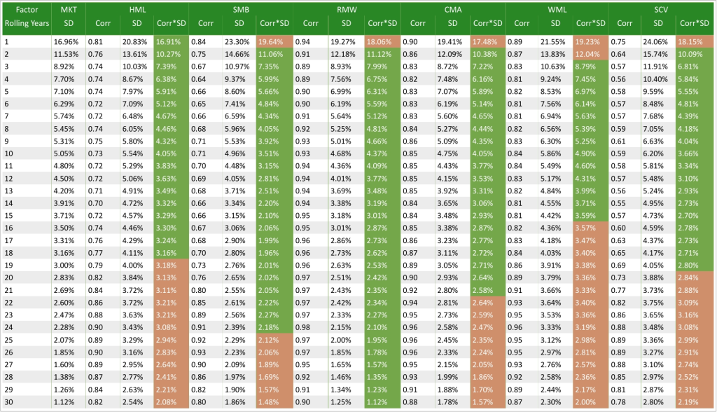
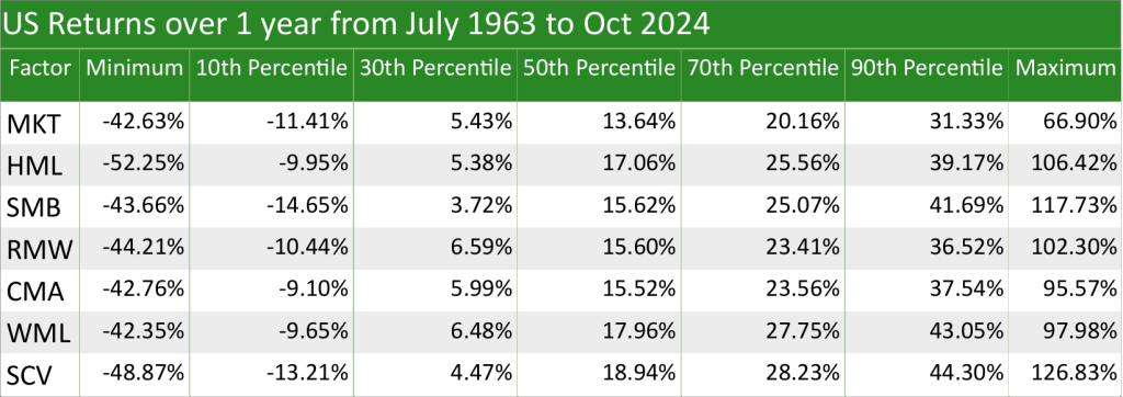
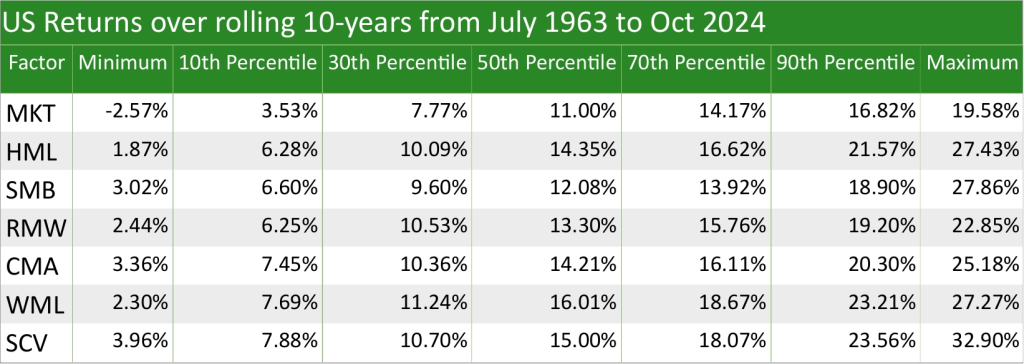
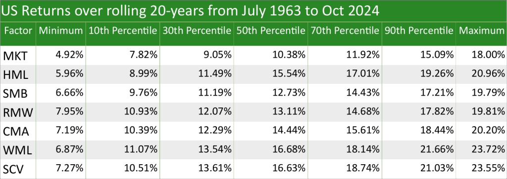
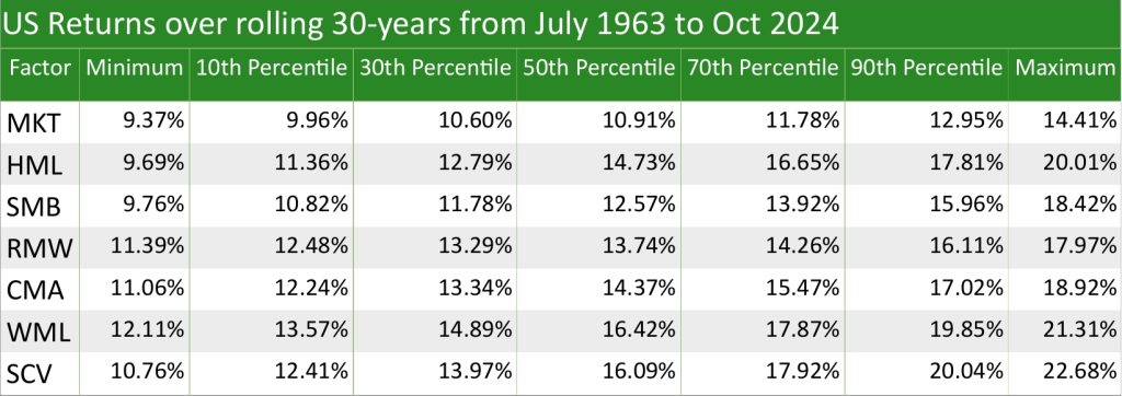
For SCV, although it doesn’t reduce a portfolio’s standard deviation with 1-year returns, surprisingly it does with rolling 2-year returns and all the way to rolling 19-year returns. For rolling 20-year returns and over, there is no reduction in portfolio standard deviation; however, this is not necessarily a bad thing, as although the range of outcomes is wider, the outcomes are more favourable compared to the Market. This is shown in the four tables below, which show US returns over 1 year, rolling 10-years, rolling 20-years, and rolling 30-years over different percentiles:
Long-only data methodology
To get long-only data, I used the same methodology from Brière and Szafarz (2016).
In Kenneth R. French’s data, Fama/French 5 Factors (2×3) are constructed long/short. To get only the long leg, we can break factors into their components and get data for those components.
Below is an example of a breakdown for the HML factor:
HML = 0.5(Small High BM + Big High BM) – 0.5(Small Low BM + Big Low BM)
We can then use the 6 Portfolios Formed on Size and Book-to-Market (2 x 3) dataset on French’s website to calculate the long leg of HML as: 0.5(SMALL HiBM+BIG HiBM), and the short leg as: 0.5(SMALL LoBM+BIG LoBM)
The same can be done for the other factors:
RMW:
- Dataset: 6 Portfolios Formed on Size and Operating Profitability (2 x 3)
- Expression: 0.5(Small High OP + Big High OP) – 0.5(Small Low OP + Big Low OP)
- Long leg: 0.5(SMALL HiOP + BIG HiOP)
- Short leg: 0.5(SMALL LoOP + BIG LoOP)
CMA:
- Dataset: 6 Portfolios Formed on Size and Investment (2 x 3)
- Expression: 0.5(Small Low INV + Big Low INV) – 0.5(Small High INV + Big High INV)
- Long leg: 0.5(SMALL LoINV + BIG LoINV)
- Short leg: 0.5(SMALL HiINV + BIG HiINV)
WML:
- Dataset: 6 Portfolios Formed on Size and Momentum (2 x 3)
- Expression: 0.5(Small High MOM + Big High MOM) – 0.5(Small Low MOM + Big Low MOM)
- Long leg: 0.5(SMALL HiPRIOR + BIG HiPRIOR)
- Short leg: 0.5(SMALL LoPRIOR + BIG LoPRIOR)
Calculating the long and short legs for SMB is done differently to neutralise bias. I copy Brière and Szafarz’s method, which they got from Fama and French (2015):
- Long leg: 1/9 x (SMALL LoBM + ME1 BM2 + SMALL HiBM + SMALL LoOP +
ME1 OP2 + SMALL HiOP + SMALL LoINV + ME1 INV2 + SMALL HiINV)
- Short leg: 1/9 x (BIG LoBM + ME2 BM2 + BIG HiBM + BIG LoOP + ME2 OP2 +
BIG HiOP + BIG LoINV + ME2 INV2 + BIG HiINV)
Finally, to get the market return, I simply used the Fama/French 5 Factors (2×3) dataset, took the Mkt-RF column, and added it with the RF column, leaving me with just Mkt.
Factor synergies
In this analysis about diversification, I’ve included small-cap value (a combination of the Size factor and Value factor) because I wanted to briefly critique ERN’s article. But it is a good time to elaborate more on SCV when it is practically synonymous with factor investing. Size and Value were the first two recognised risk-premia factors by Fama and French, which led to DFA creating a small-cap value fund. The strategy has grown more popular since, but these days when people say SCV, they typically refer to multifactor funds that include all factors in the FF6 model but have Size and Value as one of the main focuses. The idea of combining factors came from evidence that suggests combining yields better results because of higher returns, less volatility, and/or improved turnover efficiency.
For example, Value and Profitability are found to combine well together (Novy-Marx, 2013; Wahall and Repetto, 2020; Wahall and Repetto, 2021), as well as Value and Momentum (Asness et al., 2012; Fisher et al., 2016). Size historically had periods where the premium disappeared but got resurrected when filtering for Quality which includes Profitability and Investment (Asness et al., 2018; Hou and van Dijk, 2019; Rizova and Saito, 2020; Cheema et al., 2021). Although Blitz and Hanauer (2020) found filtering for Quality doesn’t resurrect the Size premium in the international market, they still found Size to pair well with other factors like Value and Momentum. Size in general gets enhanced when combined with other factors (Esakia et al., 2019).
How much to allocate to factors?
How much you allocate to factors depends entirely on your personal tastes and conviction in factors. Conviction is made up of belief and tracking variance. So a 100% allocation would be if you have full conviction in factors, while 0% would be having no conviction in factors and will stick with index funds. Both extremes can be suitable choices; however, conviction must come from you and you alone. This article so far has extensively gone through the academic papers on factor investing, but this is where we switch gears and make our own judgements based on the evidence. As Wes Gray says,
“You need to take a scientific approach to formulating an investment program/approach, but at some point you need to take a religious approach to investing and become ‘faith-based’.”
There are a number of factors that go into allocating a comfortable percentage towards factors, if at all. This includes:
- Tolerance for worse short-term volatility and drawdowns.
- Tolerance to potentially underperforming for extended periods of time.
- Added complexity and tinkering for the “perfect” portfolio.
- Doubt about premiums surviving after costs.
- Tracking error (Larry Swedroe likes to call it tracking variance, as Tracking Error is a Feature, Not a Bug).
- Keeping up with academic research and having an investment plan on how to deal with new research, something you don’t need to do if you stick with index funds.
- For any given factor, think that its existence is logical based on:
- Additional risk that compensates additional return for bearing that risk, and/or
- Mispricing due to irrational human behaviour that will persist into the foreseeable future.
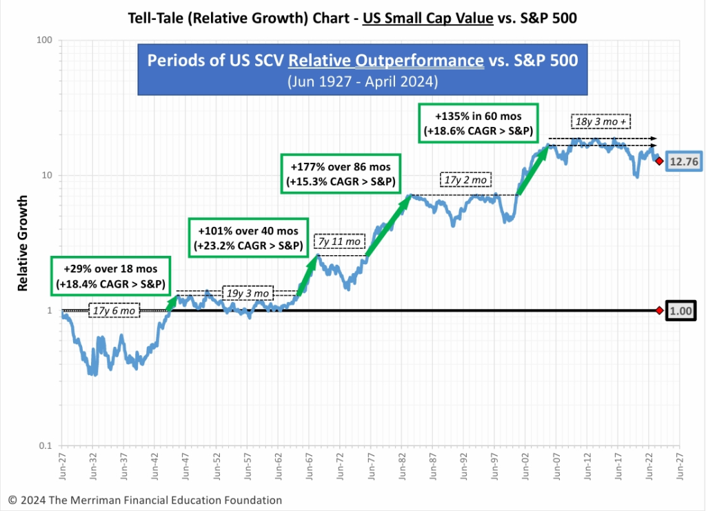
Factor investing can be a rocky road, from the uncertainty that factor investing is a viable strategy to generally worse short-term risks and potentially underperforming the market for decades, as seen in the chart below (one of the “Tell-Tale Charts” presented at the Sept 2024 Bogleheads conference). This is not made any easier when you suffer poor performance compared to just using index funds or suboptimal strategies like US concentration and sector bets.
Conclusion
For those who seek returns higher than the market, factor investing is one possible way to do so. Although we are taught to avoid active funds at all costs, factor funds sit between the two extremes of passive and active management. Factor funds actively seek returns higher than the market over the long term while having passive qualities like a transparent, rules-based methodology and a lower cost relative to active funds.
Be warned! All the good investing principles you learn for investing in index funds, like consistency and discipline, factor investing requires a mastery of those principles. Even if you stick with index funds, I hope this article at least educates you on what drives the returns of funds and markets.
For those who do pursue factor investing, know that it is an active decision. Your tolerance to this active risk to stray away from index funds, among other factors, determines how much to allocate towards factors (Vanguard, 2015). Whether you have the ability, willingness, and need for this active risk depends on your assessment of how you differ from the average investor.
So if you want exposure to risk-premia factors, what is the best way to go about it? In the next article, I talk about the fund managers that pioneered factor investing and what sets them apart from other fund managers: DFA and Avantis: The father and son of factor investing.