Geared funds: are they suitable for long-term holding?

Gearing, the act of borrowing money to invest, is commonly associated with investment properties, but can gearing be applied to stocks as well?

Fund managers like Betashares and VanEck seem to think so with their recent additions of geared ETFs available to investors. However, how gearing affects stock market returns is poorly understood by the public, and so this article attempts to explain the mechanics of gearing, address misconceptions, and see how gearing the stock market has historically performed to test the viability of the strategy.

Gearing/leverage ratio

Geared funds express how much they borrow with the gearing ratio (borrowings divided by total assets). How much a fund borrows can also be expressed by the leverage ratio (which I will refer to as leverage from now on). The following formula is used to convert the gearing ratio to leverage:

Taking the gearing ratio of 30% to 40% as an example, the leverage of the funds would be 1.43x to 1.67x, or roughly 1.5x. So, does this mean you get 1.5x returns from these funds? Yes, and no.

The compounding effect

If a fund is targeting 1.5x leverage, you only get 1.5x of the daily returns. This does not necessarily mean you get 1.5x of monthly returns, annual returns, etc. This is because of the compounding effect. For example, let’s say the daily return of an asset is 0.03% and assuming 250 trading days in a year, then the annual return is (1 + 0.03%)^250 = 7.8%. If we double the daily return to 0.06% (and assume leverage is rebalanced daily for simplicity), then the annual return becomes 16.2%, which is 2.08x rather than 2.00x. If we do the opposite and have the daily return of the asset be -0.03%, then the annual return would be -7.2%, and 2x leverage of the daily return would yield an annual return of -13.9%, or 1.93x rather than 2.00x.

So, because of the compounding effect, you get higher returns than expected with consecutive rises in price and lower returns than expected with consecutive falls in price. However, these examples assume no volatility. Let’s now consider volatility and introduce the “scary” term volatility decay or volatility drag.

Volatility decay

Volatility decay is commonly associated with the following equality:

The equality describes the return of an asset if it rose and fell by the same amount. For example, take x = 10%, so if the market rose by 10% and fell by 10%, then the return would be -1% rather than 0%. If we were to take 2x the market returns instead, then the resulting return would be -4%. That’s four times the loss! This example is the crux of the misconception that holding geared ETFs can’t be held over the long term, but is that really fair?

Any volatile asset experiences volatility decay to some extent, including unlevered ETFs. The more volatile the asset is, the more volatility decay it experiences. So, if more volatility decay is really that detrimental for long-term holding, then wouldn’t it be better to hold bonds or cash than to hold shares? Obviously, this is not the case. Despite shares being more volatile, the returns make up for it, and this can be applied to geared funds to a certain extent.
The myth that I described also gets debunked in this paper on pages 3-4: Alpha Generation and Risk Smoothing Using Managed Volatility by Tony Cooper.

Rebalancing

Another geared fund misconception is that more frequent rebalancing is undesirable because every time the fund rebalances to its target leverage, they have to either sell low or buy high. To see if rebalancing frequency really is a problem, I used gross, daily Australian returns from Jan 1997 to Dec 2024 and calculated the annualised returns with a 1.5x target leverage across different rebalancing frequencies (excluding transaction costs).

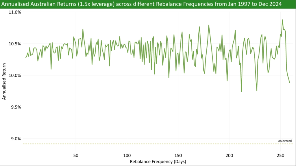
The chart suggests that there is no clear optimal rebalance frequency and that US-domiciled funds that do daily rebalancing are fine for long-term holding, especially when they don’t need to worry about transaction costs. This supports AQR’s assertion that rebalancing leveraged portfolios does not incur a drag that makes them unsuitable for long-term holding (Huss and Maloney, 2017). AQR also mentions that rebalancing can affect the distribution of returns based on the performance of the portfolio.

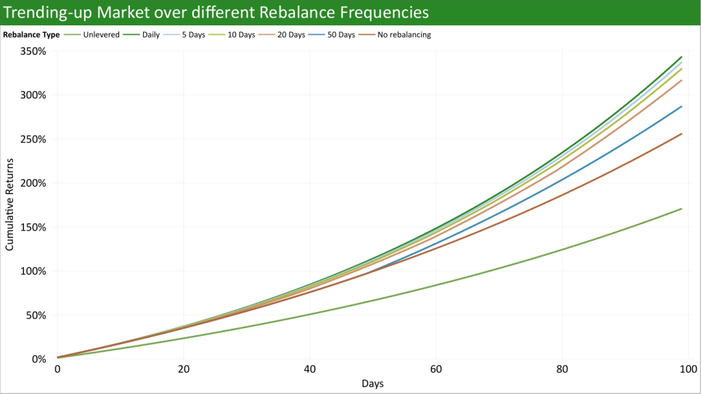
Below are simulations of how rebalancing affects returns during different types of market conditions: up-trending, down-trending, and sideways.

In a trending-up market, more frequent rebalancing is preferable to take advantage of the compounding effect.

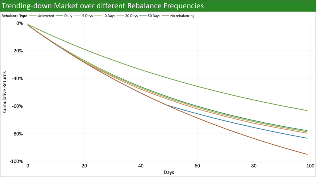
The same fact is also true in a trending-down market:

However, less frequent rebalancing is preferable in a sideways market:

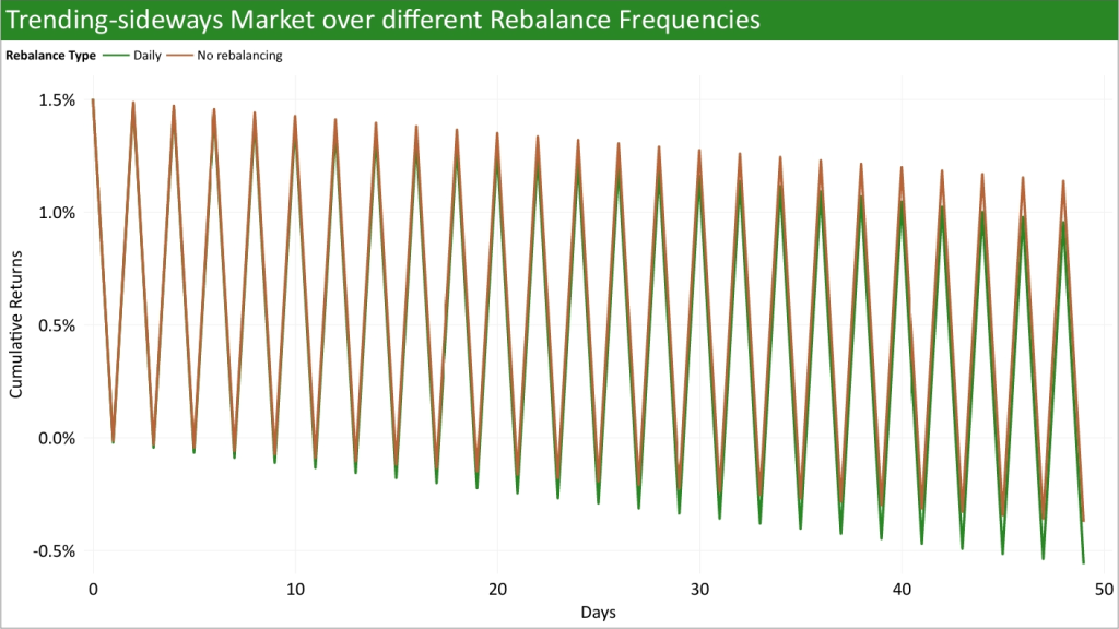
Of course, we cannot predict what type of market will happen in the future, but I just want to reiterate that rebalancing is not necessarily a bad thing as long as transaction costs are controlled.

Optimal Leverage

We’ve seen that geared funds are a viable long-term strategy, but how much leverage is too much?

To try to answer this question, I used historical Australian and International returns (MSCI Australia IMI and MSCI ACWI ex-Australia, respectively), historical RBA cash rates, added a range of borrowing spreads (borrowing rate minus RBA cash rate), and tested different MERs and transaction costs to see what was the historical optimal leverage from Jan 2001 to Dec 2024.

The funds that I’ll be trying to backtest are GHHF and CFS Geared Index Australian Share/CFS Geared Index Global Share. The reason I want to do this is because currently the only information investors can use to judge whether they should use geared funds is by its short past performance (currently 6 months for GHHF and 3 years for CFS funds). Using 24 years of data instead provides a clearer picture of how the strategy would have performed in the past and better shows the additional risk that comes with using leverage. Note that these simulations of geared funds may not be accurate because of unaccounted factors.

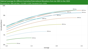
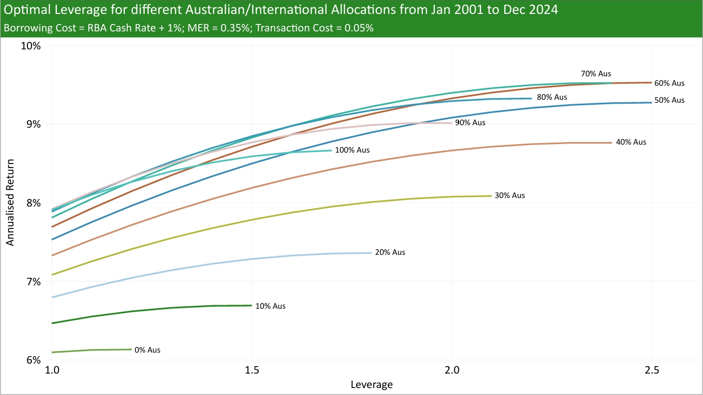
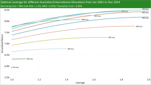
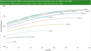
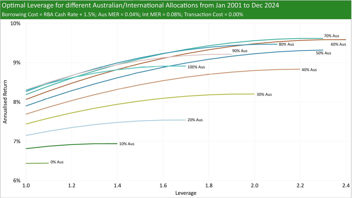
First, I’ll show charts backtesting optimal leverage using GHHF’s MER and institutional borrowing spreads, which is estimated to be around 1% to 1.5%.

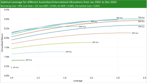
The next charts show the same but instead using CFS geared index funds’ MER plus an admin fee of 0.20%. This is to simulate holding geared funds in CFS Super, as although regulations do not allow industry super funds to borrow, Dunn et al. (2009) found that gearing in superannuation can be optimal for investors with a low risk aversion. For the record, I have chosen CFS as of the time of writing this (16/02/2025), they are the cheapest way to use geared index funds in super.

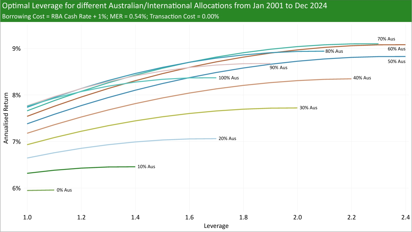
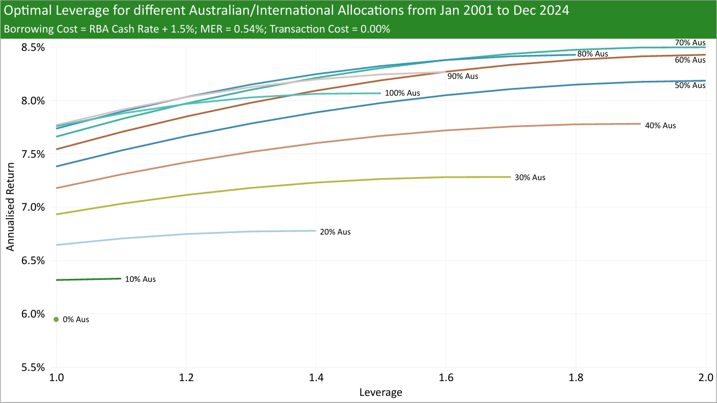
The extremely high allocation towards Australia is interesting but expected because of Australia’s dominance during this period. Using the efficient frontier on this data, the minimum standard deviation was 46% Australia and 62% Australia gave the maximum Sharpe Ratio (assuming a 3.5% risk-free rate, which was the average cash rate during the period). However, recall from my What Australian/International allocations should you choose? article that 31% Australia is the minimum standard deviation and 33% Australia gave the maximum Sharpe Ratio from 1970 to 2024.

The below charts show the scenario where one tries to do the borrowing themselves with a MER similar to A200/BGBL, but at a potentially higher rate. I show scenarios where the borrowing spread is as low as 1% and up to 3%.

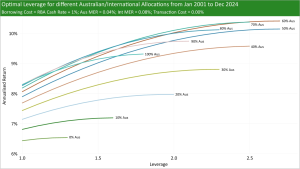
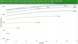
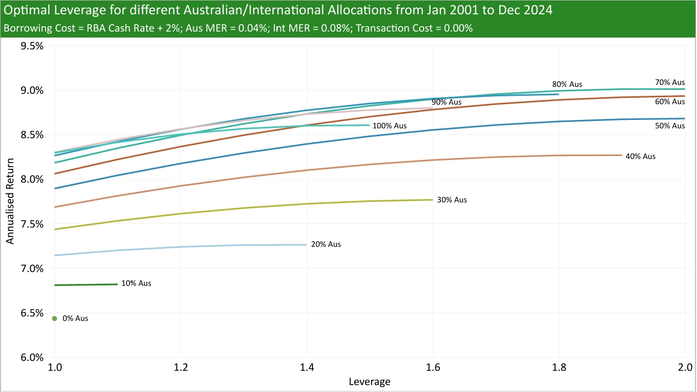
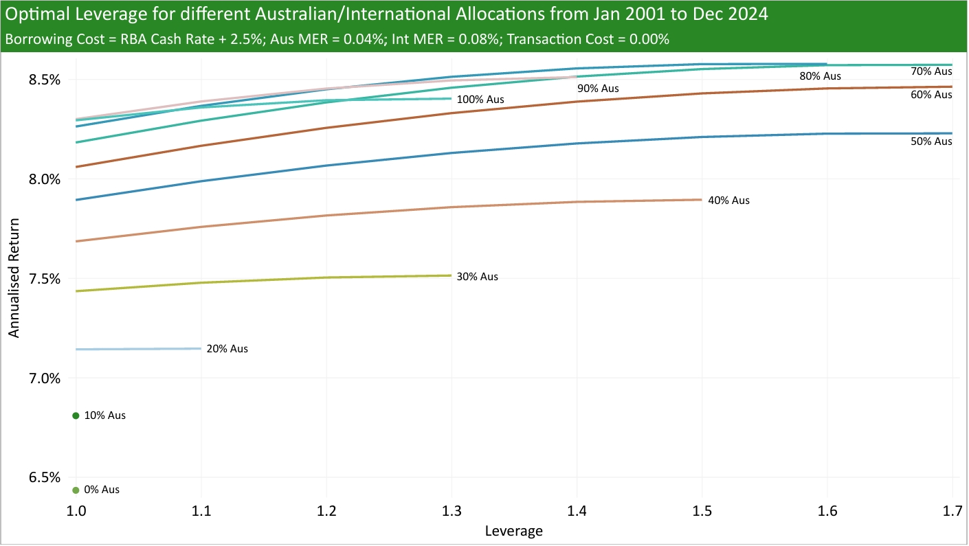
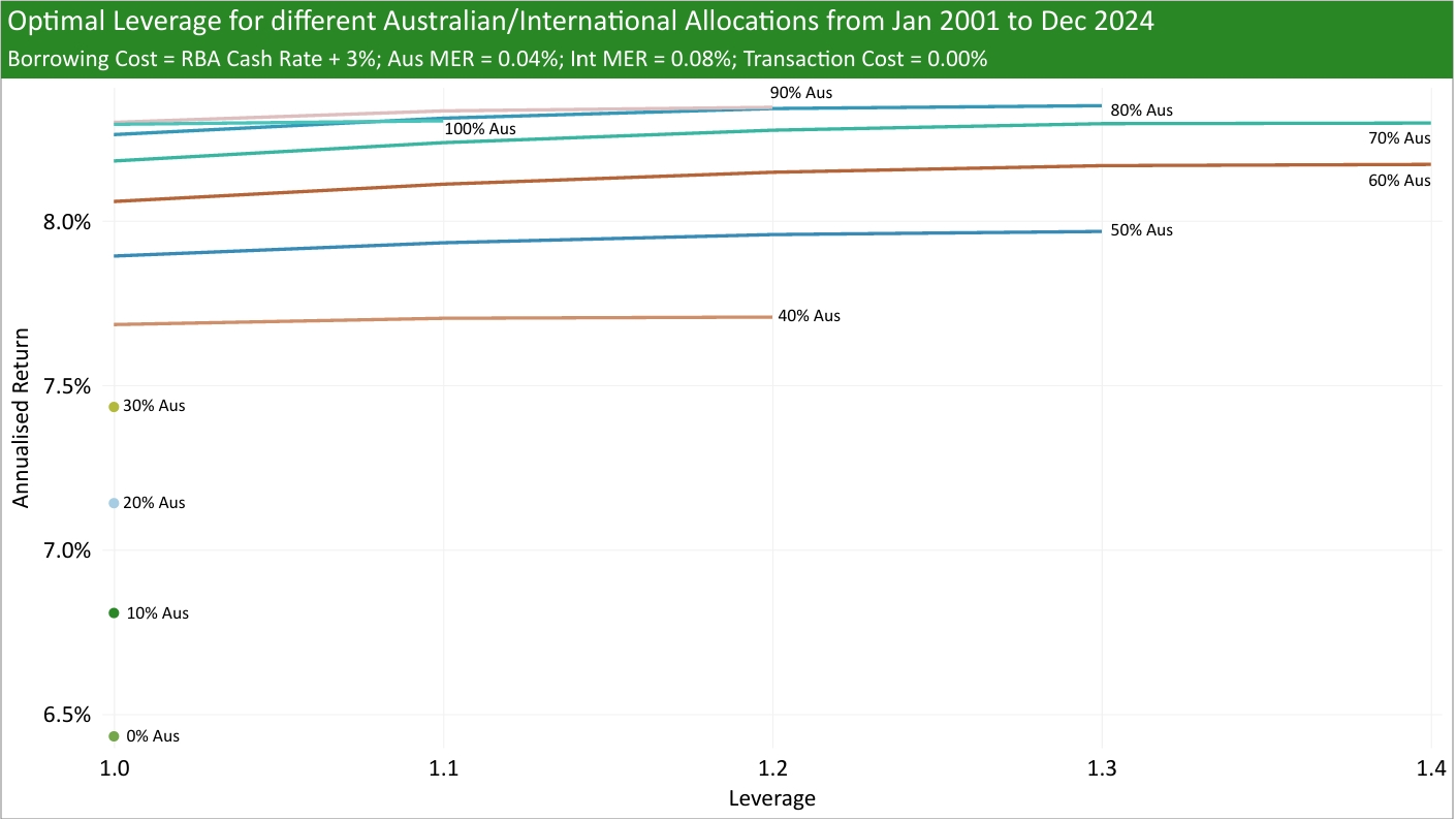
The clear takeaway from the charts is that a high borrowing spread can kill the viability of gearing. From the time period analysed, a borrowing spread above 3% makes any amount of gearing practically not feasible.

What the charts don’t account for are tax deductions from the interest cost. Geared funds can do this to a certain extent by using dividends to pay the interest cost so that investors will receive less income, mimicking a tax deduction. However, geared funds can’t use dividends to pay off all interest costs if interest costs exceed dividends. This isn’t a problem if you borrow yourself, as you can likely deduct using other taxable income.

I created a calculator to calculate the borrowing spread based on the cash rate, borrowing rate, tax rate, and dividend yield. I used the following formula:

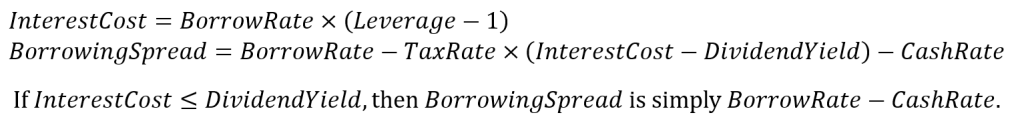
Over the time period of the data, I calculate the dividend yield to be roughly 3% based on a 35%/65% Aus/Int portfolio. Unless my formula is wrong, tax deductions seem largely a non-factor, as the dividend yield is enough to pay off the interest at a reasonable leverage. Borrowing yourself could make sense given a low enough borrowing rate and a high tax rate, but it’s going to be hard to beat geared funds that borrow at institutional rates.

Conclusion

For those seeking higher returns, using geared funds is a more approachable method compared to factor investing. Although how leverage affects stock market returns may be unintuitive at first, I hope my explanation gives you a deeper understanding of how leverage interacts with compounding, how rebalancing affects returns, and showing the historical optimal leverage over the past 24 years.

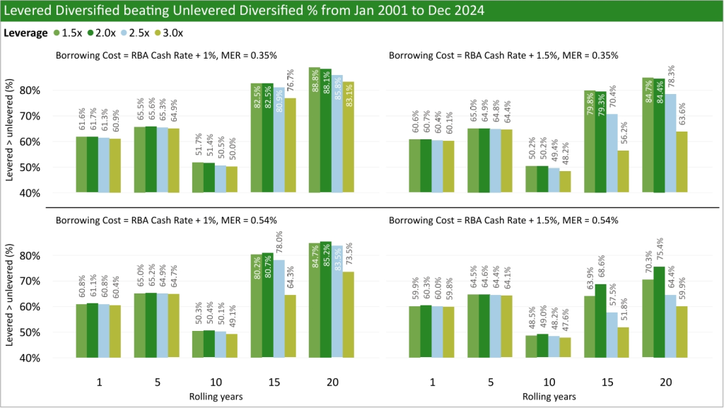
Make no mistake, using leverage means more risk, and that means potentially underperforming an unlevered portfolio. The below chart shows how often a levered, diversified portfolio (35%/65% Aus/Int) beats an unlevered, diversified portfolio over different rolling periods.

Data and Formulas

RBA Cash rate: Interest Rates and Yields – Money Market – Monthly – F1.1

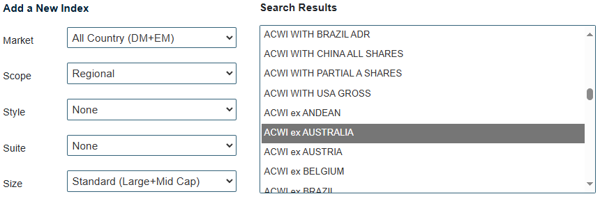
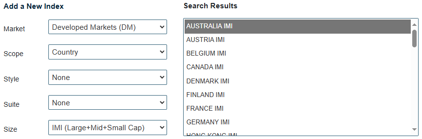
Australian and International returns: I used returns from the MSCI Australia IMI (large, mid, small-cap) index and MSCI ACWI ex-Australia index.

Instructions on how to get MSCI data:

1. Go to End of day data Regional – MSCI and click on any index name. You should arrive at this page.

2. Click Add/Remove Indexes. Remove the current index and add desired indexes. Settings I used to get my indexes:

3. Click Update Chart.

You can now configure the chart attributes and download the data with the link above the chart. However, you can only download daily data in chunks of 4-5 years this way. To get all the data, we can do some basic data scraping.

4. Right-click the page and click Inspect.

5. Click on Network, which looks like a Wi-Fi icon.

6. Click Download Data on the webpage.

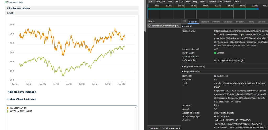
If you click on the request, you can see the API call the link made to get the data. In the request URL, you can see the chart attributes that you’ve chosen. My method of getting the data is calling the API in Python. Below is the code I used (note that the end date needs to be valid or else it will error):

import requests

# Source: https://www.msci.com/end-of-day-data-regional
# Price = STRD
# Gross = GRTR

url = "https://app2.msci.com/products/service/index/indexmaster/downloadLevelData?output=INDEX_LEVELS&currency_symbol=AUD&index_variant=GRTR&start_date=19961231&end_date=20241231&data_frequency=DAILY&baseValue=false&index_codes=664147,113648"
headers = {
    "Accept": "*/*",
    "Accept-Encoding": "gzip, deflate",
    "Accept-Language": "en-US,en;q=0.9",
    "Priority": "u=1, i",
    "Sec-Ch-Ua": "",
    "Sec-Ch-Ua-Mobile": "?0",
    "Sec-Ch-Ua-Platform": '""',
    "Sec-Fetch-Dest": "empty",
    "Sec-Fetch-Mode": "cors",
    "Sec-Fetch-Site": "same-site",
    "User-Agent": "Mozilla/5.0 (Windows NT 10.0; Win64; x64) AppleWebKit/537.36 (KHTML, like Gecko) Chrome/114.0.5735.110 Safari/537.36",
    "Cookie": "_ga=GA1.1.1145925630.1692403282; _gcl_au=1.1.115135758.1729855707; _ga_1N2VH31REP=GS1.1.1735350483.22.1.1735350488.0.0.0; OptanonConsent=isGpcEnabled=0&datestamp=Sat+Dec+28+2024+11%3A48%3A08+GMT%2B1000+(Australian+Eastern+Standard+Time)&version=202307.1.0&browserGpcFlag=0&isIABGlobal=false&hosts=&consentId=8dbe2ed7-0a67-48b3-b6e9-ae9979873187&interactionCount=1&landingPath=NotLandingPage&groups=C0001%3A1%2CC0002%3A1%2CC0003%3A1%2CC0004%3A1&AwaitingReconsent=false; _ga_763SS1MLQ7=GS1.1.1735350486.18.1.1735350491.0.0.0; mtracksessid=E042C04D184C9AB2FF6226EE57276081; _ga_73XGYWN57J=GS1.1.1735350494.1.1.1735350619.0.0.0"
}

response = requests.get(url, headers=headers)
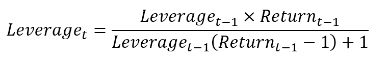
open('Data.csv', 'wb').write(response.content)

To calculate the leverage at the start of a trading day based on the leverage and return from the previous day, I used the following formula that I came up with myself:

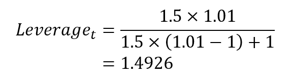
For example, if the leverage for the day was 1.5x and the unlevered return was 1%, then the following day’s leverage would be:

To calculate the return on a given day, I used the following formula: